LOGISTIC REGRESSION

> setwd("C:/Users/baron/Dropbox/627 Data Analysis/data/My data")

> Depr = read.csv("depression_data.csv")

# Another way - reading data directly from the web site:

> Depr = read.csv(url("http://fs2.american.edu/~baron/627/R/depression_data.csv"))

> names(Depr)

[1] "ID" "Gender" "Guardian_status" "Cohesion_score"

[5] "Depression_score" "Diagnosis"

> attach(Depr)

> fix(Data)

> summary(Diagnosis)

Min. 1st Qu. Median Mean 3rd Qu. Max. NA's

0.0000 0.0000 0.0000 0.1572 0.0000 1.0000 2731

# A lot of missing responses marked as NA. Omit them.

> Depr1 = na.omit(Depr)

> attach(Depr1); dim(Depr1)

[1] 458 6

# Now, fit the logistic regression model.

> fit = glm( Diagnosis ~ Gender + Guardian_status + Cohesion_score, family = binomial )

> summary(fit)

Coefficients:

Estimate Std. Error z value Pr(>|z|)

(Intercept) 1.00832 0.50478 1.998 0.04577 *

GenderMale -0.68744 0.28848 -2.383 0.01718 *

Guardian_status -0.74835 0.28602 -2.616 0.00889 **

Cohesion_score -0.04358 0.01046 -4.167 3.09e-05 ***

# All three variables are significant at 5% level, especially the cohesion score (connection to community).

# Cross-validation.

# How well does our model predict within the training data?

> Prob = fitted.values(fit)

> summary(Prob)

Min. 1st Qu. Median Mean 3rd Qu. Max.

0.01958 0.07452 0.12990 0.15720 0.21560 0.57710

# We’ll classify a student as having a depression if the probability of that exceeds 0.3.

> YesPredict = 1*(Prob > 0.3) # For all Prob > 0.3, we let YesPredict = 1.

# For all Prob <= 0.3, we let YesPredict = 0.

# Then, create a table of true and predicted responses.

> table( Diagnosis, YesPredict )

YesPredict

Diagnosis 0 1

0 359 27

1 48 24

# This is not a perfect result, there are some false positive and false negative diagnoses. Overall, we correctly predicted (359+24)/458 = 83.6% of cases. The training error rate is only 16.7%. However, among the students who are really depressed, we correctly diagnosed only 1/3.

PREDICTION ACCURACY. Training data and test data

# As we know, prediction error within the training data may be misleading since all responses were known and used to develop our classification rule. To get a fair estimate of the correct classification rate, let’s

(1) Split the data into training and test subsamples;

(2) Develop the classification rule based on the training data;

(3) Use it to classify the test data;

(4) Cross-tabulate our prediction with the true classification.

> n = length(ID)

> Z = sample(n, n/2)

> Depr.training = Depr1[ Z, ]

> Depr.testing = Depr1[ -Z, ]

# Now fit the logistic model using training data only.

> fit = glm( Diagnosis ~ Gender + Guardian_status + Cohesion_score, family = binomial, data = Depr.training )

# Use the obtained rule to classify the test data.

> Prob = predict( fit, data.frame(Depr.testing), type="response" )

> YesPredict = 1*( Prob > 0.3 )

# Cross-tabulate.

> attach(Depr.testing)

> table( YesPredict, Diagnosis )

Diagnosis

YesPredict 0 1

0 174 22

1 23 14

# We still classify 80%+ of participants correctly. However, we correctly diagnose only 39% of students who actually have depression.

Perhaps, gender, parents, and community are not enough for correct depression diagnostics.

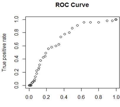
Receiver Operating Characteristic (ROC) Curve

Focus on the true positive rate and the false positive rate for different thresholds.

True positive rate = P( predict 1 | true 1 ) = power

False positive rate = P( predict 1 | true 0 ) = false alarm

> TPR = rep(0,100); FPR = rep(0,100);

> for (k in 1:100){

+ fit = glm(Diagnosis ~ Gender + Guardian_status + Cohesion_score, data=Depr1[Z,], family="binomial")

+ Prob = predict( fit, data.frame(Depr1[-Z,]), type="response" )

+ Yhat = (Prob > k/100 )

+ TPR[k] = sum( Yhat==1 & Diagnosis==1 ) / sum( Diagnosis == 1 )

+ FPR[k] = sum( Yhat==1 & Diagnosis==0 ) / sum( Diagnosis == 0 )

+ }

> plot(FPR, TPR, xlab="False positive rate", ylab="True positive rate", main="ROC curve")

> lines(FPR, TPR)

Prediction

Let’s predict the diagnosis for some particular person, a female who lives with both parents, and has an extremely weak connection with community.

> predict( fit, data.frame( Gender="Female", Guardian_status=1, Cohesion_score=26 ))

-0.8730466

# This is the predicted logit. Use the logistic function to convert it into a probability

> Y0 = predict( fit, data.frame( Gender="Female", Guardian_status=1, Cohesion_score=26 ))

> P0 = exp(Y0)/(1+exp(Y0))

> P0

0.2946208

# This can also be done by the type option.

> predict( fit, data.frame( Gender="Female", Guardian_status=1, Cohesion_score=26 ), type="response")

0.2946208

# A 29% chance of developing depression! Suppose she has an average community connection instead.

> predict( fit, data.frame( Gender="Female", Guardian_status=1, Cohesion_score=52 ), type="response")

0.1185683

# Only an 11.85% chance now.